05. Posterior Probability
Posterior Probability
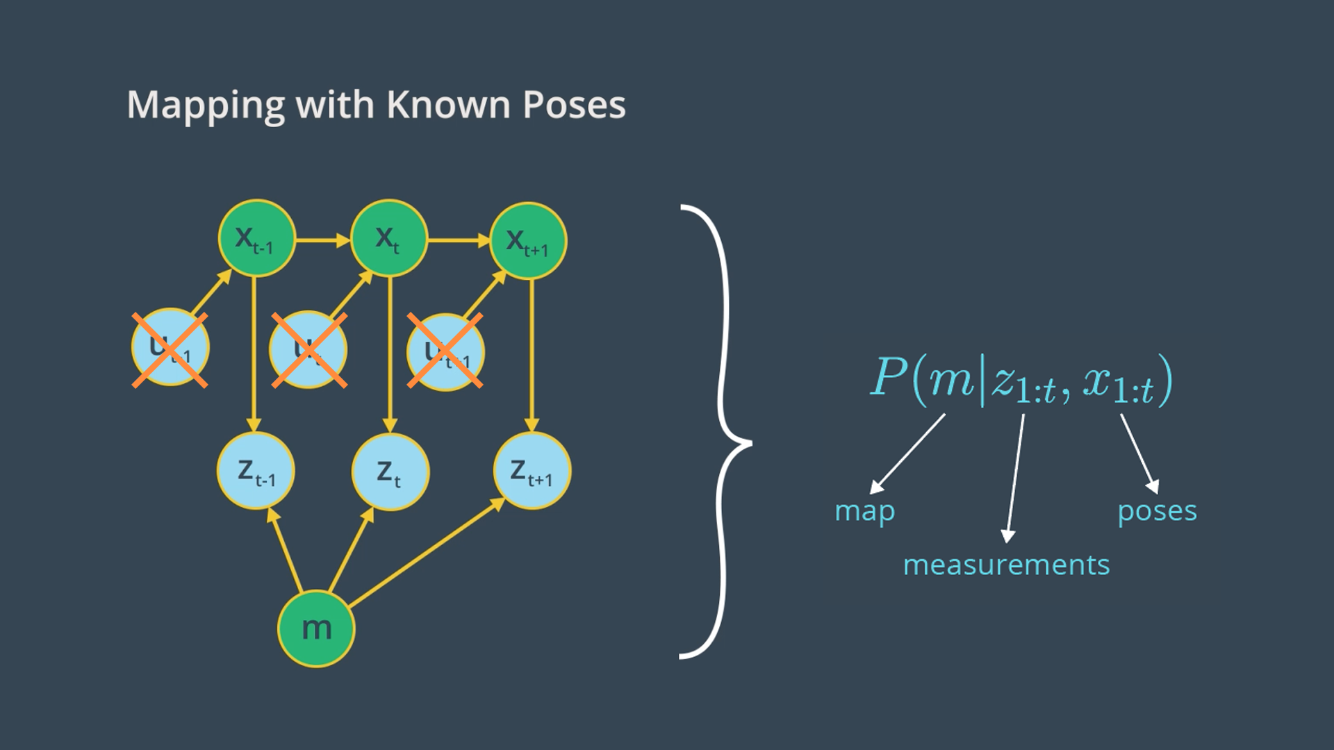
Going back to the graphical model of mapping with known poses, our goal is to implement a mapping algorithm and estimate the map given noisy measurements and assuming known poses.
The Mapping with Known Poses problem can be represented with
<span class="mathquill ud-math">P(m | z_{1:t}, x_{1:t})</span>
function. With this function, we can compute the posterior over the map given all the measurements up to time
t
and all the poses up to time
t
represented by the robot trajectory.
In estimating the map, we’ll exclude the controls u since the robot path is provided to us from SLAM. However, keep in mind that the robot controls will be included later in SLAM to estimate the robot’s trajectory.
2D Maps
For now, we will only estimate the posterior for two-dimensional maps. In the real world, a mobile robot with a two-dimensional laser rangefinder sensor is generally deployed on a flat surface to capture a slice of the 3D world. Those two-dimensional slices will be merged at each instant and partitioned into grid cells to estimate the posterior through the occupancy grid mapping algorithm. Three-dimensional maps can also be estimated through the occupancy grid algorithm, but at much higher computational memory because of the large number of noisy three-dimensional measurements that need to be filtered out.
QUIZ QUESTION: :
Match the robotic problems with their corresponding probability equations :
ANSWER CHOICES:
|
Robotic Problems |
Probability Equations |
|---|---|
|
P(x 1:t , m | z 1:t , u 1:t ) |
|
|
P(x 1:t | z 1:t , u 1:t ) |
|
|
P(m | z 1:t , x 1:t ) |
|
|
P(x 1:t | u 1:t , m , z 1:t ) |
|
|
P(x 1:t , m | z 1:t ) |
|
|
P(m | z 1:t , x 1:t , u 1:t ) |
SOLUTION:
|
Robotic Problems |
Probability Equations |
|---|---|
|
P(x 1:t , m | z 1:t , u 1:t ) |
|
|
P(m | z 1:t , x 1:t ) |
|
|
P(x 1:t | u 1:t , m , z 1:t ) |